Mixing materials

Filament and mixture

A mixture of \(n\) filaments can be represented by a stochastic row vector \(\bm{v} \in \lbrack 0,1\rbrack^{n}\) with the components specifying the fraction of each filament. More specificly, for \(n\) filaments, the mixture

\[ \bm{v}= (v_1,v_2,\dots,v_n) \]

uses a \(v_i\) fraction of the \(i\)th filament (\(i=1,2,\dots,n\)). Naturally \(v_1+v_2+\dots+v_n=1\). We use \(v_i\) as the relative speed of the \(i\)th feeding motor. We also use \(\bm{v}\) to mix the RGB chanels of colors that represent individual filaments for visualizing the mixture.

Mixing matrix

To efficiently represent and store the desired mixtures, we collect and define the vectors all at once to form a discrete, gradient palette.

When we have \(m\) mixtures over \(n\) filaments, the mixtures are stored as an \(m \times n\) mixing matrix

\[ \bm{P} = \begin{bmatrix} \bm{v}_{1} \\ \bm{v}_{2} \\ \vdots \\ \bm{v}_{m} \end{bmatrix}. \]

The matrix is a user input. If not provided, Ovenbird assumes \(m=n\) and uses a \(n \times n\) identity matrix.

Gradient mixtures

By controlling the mixing matrix, we can create a spectrum of gradient mixtures. As a minimal example, we can mix \(n=2\) filaments to create \(m=3\) mixtures using the following mixing matrix:

\[ \bm{P} = \begin{bmatrix} 1 & 0 \\ 0.5 & 0.5 \\ 0 & 1 \end{bmatrix}. \tag{1} \]

Example File

9. Multi-Material Printing → (3) Color Mixing

Mixture of mixtures

When the the extruding system change from an old mixture to a new mixture, the intermediate state is a mixture of mixtures. Consider a stochastic row vector \(\hat{\bm{u}} \in \lbrack 0,1\rbrack^{m}\) that specify the fractions of the \(m\) mixtures.

The resulting composition of the \(n\) filaments is given by the stochastic vector

\[ \bm{u} = \hat{\bm{u}}\bm{P} \in \lbrack 0,1\rbrack^{n} \tag{2} \]

For example, when \(n=2,m=3\) (as in \((1)\)) and the extruding system changes from \(\hat{\bm{u}}=(1,0,0)\) (mixture \(0\)) to \(\hat{\bm{u}}=(0,1,0)\) (mixture \(1\)), an intermediate state can be \(\hat{\bm{u}}=(0.5,0.5,0)\). From \((2)\), the composition of the filaments at this moment is

\[ \bm{u} = \hat{\bm{u}}\bm{P} =(0.75,0.25). \]

Transitional behavior

As the system changes the material mixture on the fly, it will not create distinct boundaries between the old and the new. A gradient transition is expected and modulated by the active mixing auger.

Ovenbird's Visualize Multi-Material Printing and optimization algorithms for multi-material printing with gradient transition uses a moving average model. When the feeding motor changes at travel length \(x=0\), after a delay, the material will change linearly, starting at \(x=L_1\) and finishing at \(x=L_1+L_2\). Let \(\hat{\bm{m}}(x)\) denote the motor speed represented by the fraction of mixtures, and similarly \(\hat{\bm{r}}(x)\) the resulting composition, the moving average model is

\[ \hat{\bm{r}}(x) = \frac{1}{L_{2}}\int_{x - L_{1} - L_{2}}^{x - L_{1}}\hat{\bm{m}}(x)\,\mathrm{d}x. \tag{3} \]

\(L_{1}\) is the delay length and \(L_{2}\) is the transitional length. They depend on the nozzle design and the printing speed. The resulting breakpoint between the two mixtures will be at \(x=L_1+\frac{1}{2} L_2\) where \(\hat{\bm{r}}(x)\) is the average of the two. To match the designed and resulting breakpoints we move back the breakpoints of the motors by advancement length \(L_0=L_1+\frac{1}{2}L_2\) through Move Multi-Material Breakpoints.

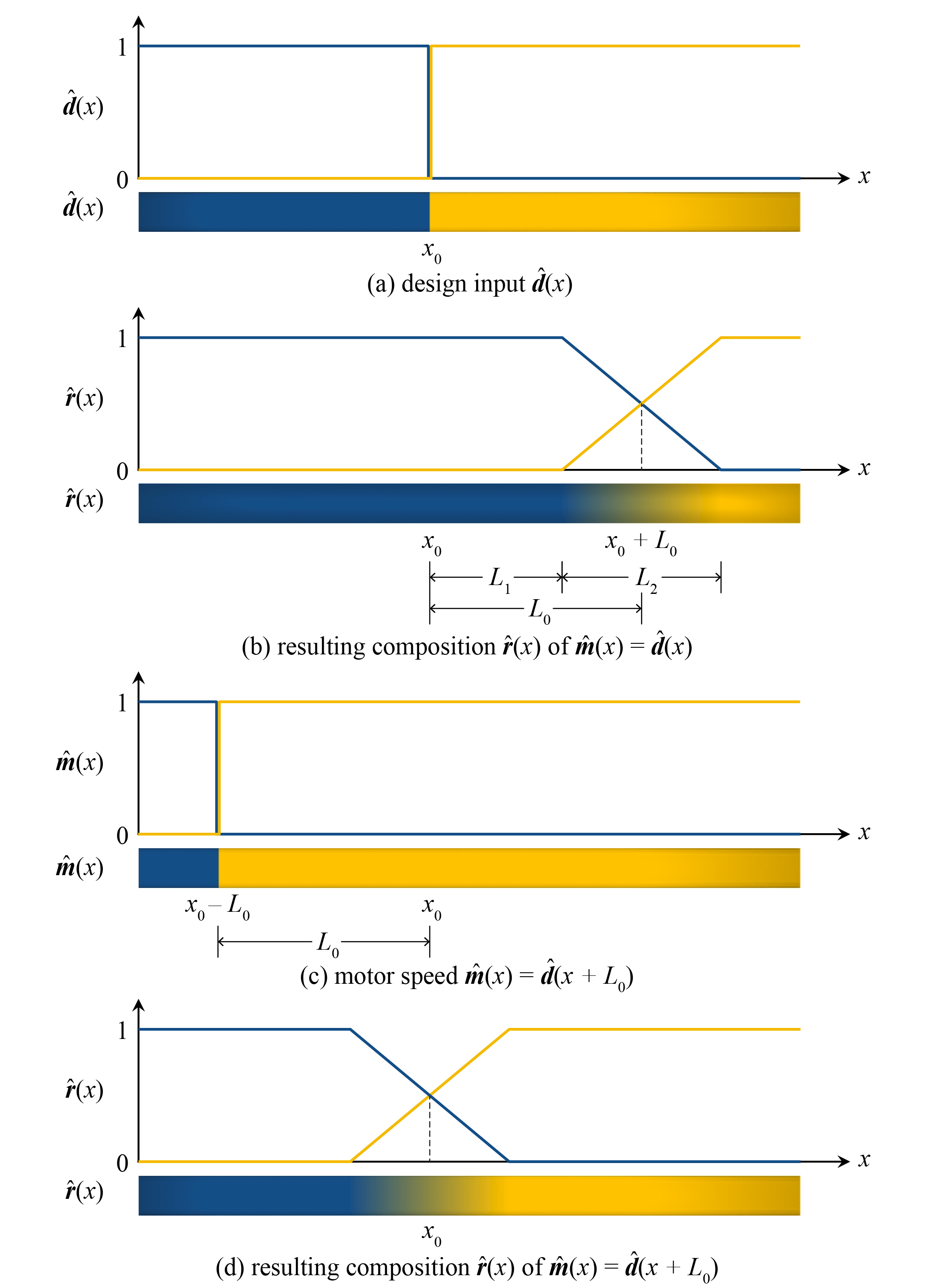
The relation between motor speed and resulting mixture composition, showing the fractions of two mixtures (components of the vector)

Another benefit of the moving average model is that we can visualize frequent changes with intervals smaller than \(L_1\) and \(L_2\).

Example Files

9. Multi-Material Printing → (4) Material Transitional Behaviors
9. Multi-Material Printing → (5) Move Breakpoints